


regionally sounds simple. Obtain the weights, begin the server, and ship requests. That works for a chatbot, however it doesn’t robotically work for an agent. In my case, I’ve been constructing an agent for automated single-cell RNA-seq evaluation. The thought is that, given uncooked knowledge, the agent can run the total pipeline by itself, deciding which instruments to name, studying the outcomes, and dealing by means of the evaluation step-by-step.
You may ask why not simply use one thing like Claude Code with a single-cell evaluation Ability. The quick reply is that for scientific workflows, that’s not fairly sufficient. Abilities are in the end prompts and may thus be overridden or ignored. Extra importantly, scientific work requires reproducibility and provenance monitoring: realizing precisely which parameters have been used, which cells have been filtered, which clustering decision produced which end result, and so on. That document must be structured and protracted, not reconstructed from a dialog. For long-running classes, you additionally want express world state administration reasonably than counting on context compaction to protect what issues. These are issues it’s important to construct intentionally. Constructing all of those on prime of a neighborhood mannequin additionally means you personal the infrastructure, and that’s what I’m going to be specializing in right here.
The agent we constructed runs on institutional HPC {hardware} utilizing latest open-weight fashions. It’s straightforward to imagine open-weight fashions usually are not sturdy sufficient for this type of work. However that’s turning into much less true. Latest releases like Qwen3.6–27B and Gemma 4–31B are genuinely helpful for structured, tool-driven workloads (In case you’re desirous about maintaining with how open supply is evolving, Interconnects AI has fascinating stuff you’ll be able to comply with). And that’s one of many foremost the explanation why native internet hosting is sensible right here. Our agent additionally helps cloud APIs like Claude and GPT, however once you use these, the entire infrastructure I’m about to explain is invisible to you. Another person has already solved it. Whenever you host the mannequin your self, these issues change into yours.
After I ran the mannequin the primary time, it labored in a slim sense. The mannequin would name instruments, the instruments would run, and the evaluation would transfer ahead. Nevertheless it wasn’t actually usable but. A easy single-cell evaluation might have 50–80 device calls in a loop. Each name carried the identical mounted baggage: the system immediate, the device schemas, and the rising dialog historical past. For this agent, the system immediate and gear schemas alone have been about 36k tokens. Earlier than the mannequin might determine something, it first needed to learn tens of 1000’s of tokens of directions and gear definitions. Then it had to try this once more on the subsequent iteration. And once more on the one after that. Every iteration took 10 to fifteen seconds. And a protracted session would finally crash out with context overflow errors, taking all of the in-memory evaluation state with it. This text is about fixing each of these issues.
The primary half covers making inference quicker by means of a set of compounding optimizations to the vLLM inference server (an open-source inference engine constructed for high-throughput LLM serving). The second half covers holding lengthy classes alive by means of higher context administration and a structured world state that survives trimming. I ran experiments on A100 and H100 GPUs to measure the affect of every change, and people are described under.
Half 1: Making Inference Quick
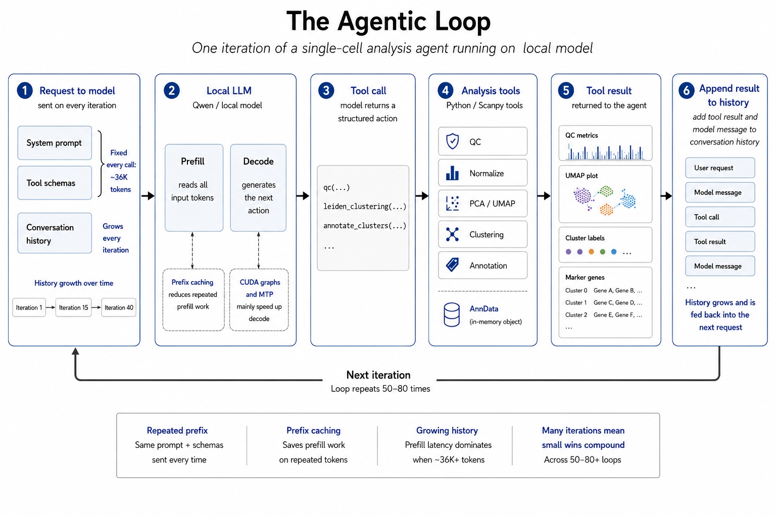
Earlier than stepping into the person optimizations, it helps to know what’s truly taking place on every iteration of the agent loop. The diagram under exhibits a single iteration: the agent sends a request containing the system immediate, device schemas, and the total dialog historical past to the mannequin. The mannequin reads all of it and decides which instruments to name. The device runs and returns a end result, and that end result will get appended to the historical past earlier than the subsequent iteration begins. Two issues are price noting right here. The mounted prefix, which is the system immediate plus device schemas, is roughly 36k tokens and will get despatched on each single name. And the dialog historical past grows with each iteration. By iteration 40, the mannequin is not studying a brief instruction. It’s studying a protracted evaluation transcript with many device calls, device outputs, intermediate outcomes, and so on. Each of these items have an effect on the efficiency of the agent.
1.1 CUDA Graphs: Lowering A whole bunch of Directions Per Token to One
To know this one, it helps to know what occurs inside a GPU when it generates a single token.
Producing a single token in the course of the decode part entails executing a sequence of GPU kernels so as: consideration, feed-forward, normalization, and so forth. Every of those kernel launchers has a small coordination price on the CPU facet. The CPU has to queue an instruction telling the GPU precisely which kernel to run, with which tensor shapes and reminiscence pointers. For a 27-billion-parameter mannequin we’ve been working with, this implies a whole lot of particular person dispatches per token. Each is small, however they add up.
CUDA graphs remove this overhead. Earlier than dealing with any actual requests, vLLM can run a warmup go the place it information all of the kernel dispatches for the decode step into one single replayable object. After that, producing every token is one instruction to the GPU as a substitute of a whole lot. The result’s roughly 20–25% decrease latency from this single change, with no change to the mannequin itself.
That is nice, however CUDA graphs additionally require static tensor shapes, that means the graph is compiled for a selected batch measurement and sequence size. What this implies for us is that the primary startup takes longer than subsequent ones. Subsequent startups are a lot quicker. As proven in Determine 8 under, for an agent working a whole lot of iterations, the cumulative impact is lots.
1.2 Becoming Extra in Reminiscence
Each weight in a neural community is a quantity, and the format you employ to retailer that quantity impacts each how a lot reminiscence it takes and how briskly the GPU can work with it. The usual format for contemporary LLMs (a minimum of for coaching) is BF16, which shops every weight as a 16-bit floating quantity. For Qwen3.6–27B’s 27 billion parameters, that’s roughly 56GB of weight knowledge simply to load the mannequin.
FP8 shops every weight in a single byte as a substitute of two. The identical mannequin now matches in round 31GB. We are able to now use that freed reminiscence for the KV cache, which is what shops the dialog context. Extra KV cache means the mannequin can deal with longer inputs earlier than working out of room. However the reminiscence we free for the KV cache isn’t used the identical means by each mannequin. How a lot precise context we get from that reminiscence depends upon the mannequin structure itself. A helpful quantity right here is KV reminiscence per token, which is simply mainly how a lot GPU reminiscence the mannequin must retailer one token of context.
Because of this two fashions with comparable parameter counts can behave in another way in apply. For instance, Gemma 4–31B makes use of roughly 1.1MB of KV cache per token. Qwen3.6–27B, relying on the way you rely its consideration layers, could be nearer to 256KB per token in a conservative estimate. Meaning the identical quantity of leftover GPU buys you a lot extra tokens of context on Qwen than on Gemma.
For instance, suppose after loading the mannequin on two 80GB GPUs and leaving some runtime overhead, we now have round 82GB obtainable for the KV cache. With Gemma, we get 82GB/1.1MB ≈ 74k tokens. With Qwen, if we use 256KB per token, 82GB/256KB ≈ 320k tokens. In apply, the mannequin’s configured most context size caps this round 262k tokens (properly, truly, in the event you use YaRN, it may be prolonged to 1M tokens), however the level is similar. Qwen can use the identical GPU reminiscence far more effectively for lengthy context workloads.
Going again to working with FP8 for our mannequin weights, truly multiplying FP8 numbers collectively utilizing {hardware} tensor cores requires devoted FP8 arithmetic items, which NVIDIA launched within the Hopper era. The H100 has them. The A100 doesn’t. So on A100 we use BF16 weights, and on H100 we use FP8 weights. The velocity profit follows straight from this. Throughout decode, the GPU has to learn the mannequin weights from reminiscence on each single token it generates. At batch measurement 1, which is what a single-user agent session appears like, that reminiscence studying is the bottleneck, not the computation itself. Smaller weights imply much less knowledge to learn per token, which implies quicker era.
Aside from the mannequin weights themselves, there’s a second place the place FP8 helps, and this one works on each GPUs. Storing KV cache vectors in FP8 as a substitute of BF16 halves the per-token price (for Qwen3.6–27B, it goes from 256KB to 128KB), straight doubling what number of tokens slot in reminiscence. The vectors are saved in FP8 for reminiscence effectivity however dequantized again to BF16 when truly utilized in consideration computation, so this doesn’t require FP8 tensor cores.

There’s yet one more factor that compounds the reminiscence profit. Operating the mannequin throughout a number of GPUs with tensor parallelism splits the burden matrices throughout each playing cards. Every GPU now holds half the weights, which frees up much more room per GPU for KV cache. On A100, this takes the per-GPU weight footprint from 56GB all the way down to 28GB, leaving 44GB per GPU for KV cache as a substitute of 16GB. That interprets to a context window of round 180K tokens on A100 {hardware}, which is sufficient for a full evaluation session to run with out overflow (Tensor parallelism is totally different from FSDP, which is one other technique of distributing workload. You possibly can learn my different article here to be taught extra).

1.3 Prefix Caching
Do not forget that mounted prefix we talked about earlier: the system immediate and gear schemas that get despatched on each single agent loop iteration. For this agent, that’s roughly 36K tokens. On each iteration, earlier than the mannequin can determine something, it first has to learn and course of all of these tokens from scratch. Meaning computing the total consideration over 36K tokens on each name, despite the fact that nothing in that prefix has modified because the final name.
Prefix caching solves this by storing the important thing and worth vectors for any token sequence the mannequin has already processed. If the subsequent request begins with the identical prefix, these vectors are retrieved straight from cache reasonably than recomputed. The mannequin solely pays the total prefill price on the very first request. Each subsequent request in the identical session skips straight to the brand new tokens on the tail. But when one thing modifications in that prefix mid-way by means of the session, the complete historical past must be learn from scratch. For instance, in the event you edit the system immediate or edit the device checklist by including MCP instruments, as an illustration, the entire thing must be re-read. The identical is true in the event you change the mannequin mid-session. You may need seen this in Claude Code the place it tells you that the complete message must be re-read in the event you attempt to change the mannequin mid-session.
For an agent loop, that is significantly helpful as a result of the mounted portion is massive and the brand new portion added every iteration is relatively small. Because the session progresses, the cache hit charge truly improves. By iteration 40, many of the request is cached historical past and solely the latest additions want contemporary computation.

To measure the precise affect, we ran the agent’s actual system immediate and gear schemas, the total 36K tokens, by means of the vLLM server with and with out prefix caching enabled, throughout each A100 and H100 {hardware}. We measured time to first token on the chilly begin, which is the primary request the place the cache is empty and the total prefix needs to be computed from scratch, and on subsequent heat requests the place the cache is already populated. On A100, chilly begin Time to First Token (TTFT) was 11,470ms. With a heat cache, that dropped to 706ms. On H100, the chilly begin was 2,655ms, dropping to 249ms on heat begin. That’s as a result of the prefix isn’t being recomputed. Solely the brand new tokens on the tail are processed.

1.4 Speculative Decoding
Decoding is inherently sequential. The mannequin generates one token, appends it to the context, then generates the subsequent in an autoregressive method. Every token depends upon all those earlier than it, so you can’t parallelize throughout tokens the best way you’ll be able to parallelize throughout a batch. For a single-user agent session at batch measurement 1, this sequential bottleneck is the principle constraint on throughput.
Speculative decoding will get round this by introducing a small draft mannequin that runs forward of the principle mannequin. The draft mannequin proposes the subsequent okay tokens cheaply and rapidly. The principle mannequin then verifies all okay proposed tokens in a single parallel ahead go. As a result of the principle mannequin is studying okay tokens concurrently reasonably than producing them one after the other, the verification step prices roughly the identical as producing a single token usually. If many of the proposals are accepted, you get okay tokens for almost the value of 1.

The important thing variable is the acceptance charge. If the draft mannequin’s proposals are constantly unsuitable, the principle mannequin rejects them and falls again to producing one token at a time, however you continue to paid the overhead of working the draft path. The precise breakeven level depends upon the draft mannequin, the variety of proposed tokens, the {hardware}, and the serving implementation. In our setup, acceptance under roughly 40% was not price it.
That is the place the selection of draft mannequin issues lots. We initially tried DFlash, a separate small mannequin used as a draft. The acceptance charge on our workload was 4 to 7%, properly under breakeven. It truly made issues slower. (To be truthful, as of the day I’m writing this text, the creators of DFlash over at Z lab stated that the draft mannequin from Qwen3.6–27B was still under training, so it is likely to be higher as soon as that’s finished). However for our case, Qwen3.6–27B has one thing higher in-built: a Multi-Token Prediction head (MTP), which is an auxiliary prediction head skilled alongside the principle mannequin and baked straight into the weights. As a result of the MTP head is skilled alongside the principle mannequin and makes use of the mannequin’s personal hidden states, its proposals are significantly better aligned with what the mannequin would have generated anyway.
We measured MTP acceptance charges throughout actual agent classes on each A100 and H100. At a median ~89% acceptance, MTP was safely on the helpful facet of the tradeoff. Properly above breakeven, and steady throughout totally different elements of the evaluation workflow.

Placing It All Collectively
Every of those optimizations was benchmarked cumulatively, with each configuration constructing on all of the earlier ones. The complete stack was measured throughout each A100 and H100 {hardware} on the Qwen mannequin we’ve been utilizing with our actual 36K token system immediate, matching the precise situations of an agent session.

A number of issues stand out. CUDA graphs are the dominant decode acquire, giving roughly 3x on A100 and 6x on H100. The H100 baseline truly begins slower than A100, which is counterintuitive (truly, one factor to notice right here is that the communication protocol between your GPUs issues lots, aside from simply the GPU kind. The gold normal is utilizing NVLink by way of NVSwitch adopted by NVLink Bridge, after which PCIe). It displays how severely CPU dispatch overhead limits FP8 kernels earlier than graphs are compiled. As soon as graphs are enabled, although, H100 pulls forward and stays there.
FP8 KV cache and prefix caching are flat on decode throughput, which is anticipated. They deal with reminiscence capability and prefill latency respectively, not token era velocity. The prefix caching impact exhibits up clearly on the TTFT facet of the waterfall: a flat line throughout the primary three configurations, then a pointy drop when caching is enabled.
MTP is the second largest decode contributor on each GPUs, including round 37% on A100 and 20% on H100.
Half 2: Preserving Lengthy Classes Alive
When utilizing cloud fashions, context administration is simpler to disregard. The context home windows are sometimes massive sufficient for abnormal chat classes, and the serving infrastructure is dealt with for you. Whenever you run a neighborhood mannequin, the context window turns into a {hardware} finances. Extra context means extra KV cache. Extra KV cache means extra GPU reminiscence. On considered one of our earlier A100 configurations, the efficient context window was round 74K tokens.
A single-cell evaluation can run 50 to 80+ iterations. Every iteration appends device calls, device outcomes, intermediate observations, plots, errors, corrections, and person constraints again into the dialog historical past. When it fills with none administration, the API returns a context size exceeded error and the session dies, taking all of the in-memory evaluation state with it, together with the AnnData object holding the processed dataset.
So the issue was not simply making the mannequin quick. The agent additionally wanted to outlive lengthy sufficient to complete.
Context administration sounds easy. Observe how full the window is and trim it when it will get too full. In apply, although, there are a couple of locations the place naive implementations can go unsuitable.
Anthropic has a cookbook on context engineering for agents, and describes three methods for long-horizon duties: compaction, structured note-taking, and multi-agent architectures. Compaction is the commonest answer, and for a general-purpose assistant, it really works properly. When the context fills up, the dialog historical past is handed again to the mannequin to summarize, and the session continues with that compressed model.
For a common assistant, that may work. For scientific evaluation, it loses the unsuitable issues.
The issue for a scientific workflow is {that a} prose abstract loses precisely the data you want. “The evaluation clustered the info and ran high quality management” is a legitimate abstract, however it discards the QC thresholds, the clustering decision, the variety of cells retained, and so on. These actual parameters are what the agent wants to breed a step, describe its methodology, or accurately reply a query about what it did. These usually are not beauty particulars. They’re the evaluation. A scientific agent wants the precise document, not simply the gist.
Past the conceptual downside with compaction, there are extra fundamental methods context administration can fail. The primary is fixed-cost accounting. Each API name contains the system immediate, device schemas, and reserved completion finances earlier than a single historical past message seems. For this agent, the system immediate and gear schemas alone are round 36K tokens. If the trim threshold doesn’t subtract these mounted prices first, the agent can find yourself trimming towards a finances that was already exceeded earlier than any historical past was included.
Past the conceptual downside with compaction, there are extra fundamental methods context administration can fail. The primary is fixed-cost accounting. Each API name contains the system immediate, device schemas, and reserved completion finances earlier than a single historical past message seems. For this agent, the system immediate and gear schemas alone are round 36K tokens. If the trim threshold doesn’t subtract these mounted prices first, the agent can find yourself trimming towards a finances that was already exceeded earlier than any historical past was included.
The third is context-limit discovery. The context restrict is the denominator of each finances calculation. If the mannequin metadata question fails and the code silently falls again to a hardcoded default, each trim choice downstream is unsuitable.
The higher strategy is to cease treating the dialog historical past because the document of what occurred. For a scientific workflow, you have already got a extra dependable document: the structured log of each step the agent took, with actual parameters and outcomes. We name this the world state.
The world state is a Python object that tracks the evaluation because it progresses. Each device name that completes writes a structured entry to it: which step ran, with what parameters, and what the outcomes have been. This will get serialized into the system immediate on each iteration. It takes below 1,000 tokens, it incorporates the precise parameters reasonably than a prose abstract of them, and it lives within the system immediate, which is rarely trimmed. When outdated device outcomes are faraway from the message historical past, the evaluation document survives intact.
This modifications how you concentrate on trimming. As a substitute of treating message historical past as one thing treasured that needs to be preserved as a result of it incorporates the document of what occurred, you’ll be able to trim it aggressively as a result of the document is elsewhere. The historical past turns into a helpful context. The world state turns into the bottom reality.

The world state handles the query of what to protect. The remaining fixes deal with the query of learn how to know when to trim and by how a lot.

The primary repair was to cease treating the complete context window as obtainable historical past. The obtainable finances is computed by subtracting mounted prices upfront:
obtainable = (
    context_limit
    - tool_schema_tokens
    - system_tokens
    - COMPLETION_RESERVE
    - safety_margin
)
With a 262K context window and typical overhead, this leaves round 219K tokens for message historical past. With a tighter 32K context, it accurately experiences just a few thousand tokens obtainable. That’s helpful. It tells you instantly that lengthy classes received’t work at that context measurement, as a substitute of silently crashing 3 iterations later.
The second repair was self-calibrating token counts. Slightly than attempting to match Qwen’s actual tokenization guidelines, we use the API’s personal response to appropriate our estimates. After each name, the response contains the precise variety of tokens processed. We evaluate that to our estimate and modify the right issue upward if the precise rely was increased:
if actual_tokens > our_estimate:
    calibration = max(calibration, actual_tokens / our_estimate)
    calibration = min(calibration, 4.0)
The issue solely goes up. An overestimate causes barely extra frequent trimming. An underestimate causes the subsequent name to fail. The results are uneven, so the correction is one-directional.
The third repair was to trim strategically reasonably than uniformly. When approaching the finances, the agent collects eligible device outcomes, types them by measurement, and removes the most important ones first. A single massive code execution output can comprise 50 to 200KB of logs, tables, or base64-encoded plot knowledge. Eradicating one massive block can save as a lot context as eradicating dozens of small messages. Person messages are by no means trimmed. They comprise the scientific intent and constraints that outline what the evaluation is meant to do.
Collectively, these modifications made the agent truly usable. A full 50+ iteration evaluation now runs to completion with out the person seeing a context error.
Conclusion
Operating an LLM regionally for an actual agentic workload exposes issues which might be straightforward to overlook when utilizing a cloud API. The mannequin doesn’t simply should be good. The inference server must be configured intentionally, and the context window must be managed intentionally. Neither downside is unattainable, however neither is computerized.
The optimizations in Half 1 compound in methods that aren’t apparent upfront. CUDA graphs take a barely useful baseline and make it usable. Prefix caching modifications the interactive really feel of the agent by avoiding the price of rereading the identical 36K-token prefix on each name. FP8 KV cache will increase the quantity of context that matches in reminiscence. MTP provides significant decode throughput on prime. Collectively, these modifications take the agent from 10 to fifteen seconds per iteration to roughly 1 to three seconds.
The context administration modifications in Half 2 resolve a distinct downside: correctness. An extended-running scientific agent wants to recollect what it did, not simply proceed the dialog. The dialog historical past is a helpful context, however it’s a fragile supply of reality. It grows, will get trimmed, and finally needs to be compressed or discarded. The world state strategy, specifically, is one thing I might suggest to anybody constructing a domain-specific agent for scientific or analytical workflows. The sturdy document ought to reside exterior the transcript, in a structured state that information every step with actual parameters and outcomes.
That was the principle lesson from constructing this technique. A helpful agent isn’t just an LLM with instruments. It’s a loop with infrastructure round it. The mannequin decides what to do subsequent, however the system round it determines whether or not the loop is quick sufficient, steady sufficient, and dependable sufficient to complete the work.
Thanks for studying, and I hope you discovered this beneficial!
