


Quantum Mechanics is a elementary idea in physics that explains phenomena at a microscopic scale (like atoms and subatomic particles). This “new” (1900) area differs from Classical Physics, which describes nature at a macroscopic scale (like our bodies and machines) and doesn’t apply on the quantum stage.
Quantum Computing is the exploitation of properties of Quantum Mechanics to carry out computations and remedy issues {that a} classical pc can’t and by no means will.
Regular computer systems communicate the binary code language: they assign a sample of binary digits (1s and 0s) to every character and instruction, and retailer and course of that info in bits. Even your Python code is translated into binary digits when it runs in your laptop computer. For instance:
The phrase “Hello” → “h”: 01001000 and “i”: 01101001 → 01001000 01101001
On the opposite finish, quantum computer systems course of info with qubits (quantum bits), which may be each 0 and 1 on the identical time. That makes quantum machines dramatically quicker than regular ones for particular issues (i.e. probabilistic computation).
Quantum Computer systems
Quantum computer systems use atoms and electrons, as a substitute of classical silicon-based chips. In consequence, they will leverage Quantum Mechanics to carry out calculations a lot quicker than regular machines. For example, 8-bits is sufficient for a classical pc to characterize any quantity between 0 and 255, however 8-qubits is sufficient for a quantum pc to characterize each quantity between 0 and 255 on the identical time. A couple of hundred qubits can be sufficient to characterize extra numbers than there are atoms within the universe.
The mind of a quantum pc is a tiny qubit chip fabricated from metals or sapphire.
Nevertheless, probably the most iconic half is the massive cooling {hardware} fabricated from gold that appears like a chandelier hanging inside a metal cylinder: the dilution fridge. It cools the chip to a temperature colder than outer area as warmth destroys quantum states (mainly the colder it’s, the extra correct it will get).
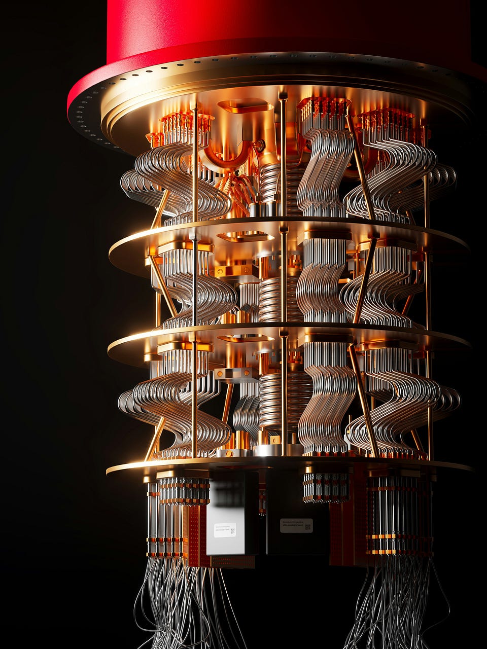
That’s the main sort of structure, and it’s known as superconducting-qubits: synthetic atoms created from circuits utilizing superconductors (like aluminum) that exhibit zero electrical resistance at ultra-low temperatures. An alternate structure is ion-traps (charged atoms trapped in electromagnetic fields in extremely‑excessive vacuum), which is extra correct however slower than the previous.
There isn’t a actual public rely of what number of quantum computer systems are on the market, however estimates are round 200 worldwide. As of immediately, probably the most superior ones are:
- IBM’s Condor, the most important qubit rely constructed thus far (1000 qubits), even when that alone doesn’t equal helpful computation as error charges nonetheless matter.
- Google’s Willow (105 qubits), with good error price however nonetheless removed from fault‑tolerant giant‑scale computing.
- IonQ’s Tempo (100 qubits), ion-traps quantum pc with good capabilities however nonetheless slower than superconducting machines.
- Quantinuum’s Helios (98 qubits), makes use of ion-traps structure with a few of the highest accuracy reported immediately.
- Rigetti Computing’s Ankaa (80 qubits).
- Intel’s Tunnel Falls (12 qubits).
- Canada Xanadu’s Aurora (12 qubits), the primary photonic quantum pc, utilizing gentle as a substitute of electrons to course of info.
- Microsoft’s Majorana, the primary pc designed to scale to one million qubits on a single chip (however it has 8 qubits in the mean time).
- Chinese language SpinQ’s Mini, the primary transportable small-scale quantum pc (2 qubits).
- NVIDIA’s QPU (Quantum Processing Unit), the primary GPU-accelerated quantum system.
For the time being, it’s unimaginable for a traditional particular person to personal a large-scale quantum pc, however you’ll be able to entry them by way of the cloud.
Setup
In Python, there are a number of libraries to work with quantum computer systems all over the world:
- Qiskit by IBM is probably the most full high-level ecosystem for working quantum packages on IBM quantum computer systems, excellent for rookies.
- Cirq by Google, devoted to low-level management on their {hardware}, extra fitted to analysis.
- PennyLane by Xanadu makes a speciality of Quantum Machine Studying, it runs on their proprietary photonic computer systems however it may possibly hook up with different suppliers too.
- ProjectQ by ETH Zurich College, an open-source mission that’s making an attempt to grow to be the primary general-purpose package deal for quantum computing.
For this tutorial, I shall use IBM’s Qiskit because it’s the trade chief (pip set up qiskit).
Probably the most primary code we are able to write is to create a quantum circuit (surroundings for quantum computation) with just one qubit and initialize it as 0. To be able to measure the state of the qubit, we want a statevector, which mainly tells you the present quantum actuality of your circuit.
from qiskit import QuantumCircuit
from qiskit.quantum_info import Statevector

q = QuantumCircuit(1,0) #circuit with 1 quantum bit and 0 traditional bit
state = Statevector.from_instruction(q) #measure state
state.chances() #print prob%
It means: the chance that the qubit is 0 (first component) is 100%, whereas the chance that the qubit is 1 (second component) is 0%. You may print it like this:
print(f"[q=0 {round(state.probabilities()[0]*100)}%,
         q=1 {spherical(state.chances()[1]*100)}%]")
Let’s visualize the state:
from qiskit.visualization import plot_bloch_multivector

plot_bloch_multivector(state, figsize=(3,3))
As you’ll be able to see from the 3D illustration of the quantum state, the qubit is 100% at 0. That was the quantum equal of “whats up world“, and now we are able to transfer on to the quantum equal of “1+1=2“.
Qubits
Qubits have two elementary properties of Quantum Mechanics: Superposition and Entanglement.
Superposition — classical bits may be both 1 or 0, however by no means each. Quite the opposite, a qubit may be each (technically it’s a linear mixture of an infinite variety of states between 1 and 0), and solely when measured, the superposition collapses to 1 or 0 and stays like that without end. It’s because the act of observing a quantum particle forces it to tackle a classical binary state of both 1 or 0 (mainly the story of Schrödinger’s cat that everyone knows and love). Due to this fact, a qubit has a sure chance of collapsing to 1 or 0.
q = QuantumCircuit(1,0)
q.h(0) #add Superposition
state = Statevector.from_instruction(q)
print(f"[q=0 {round(state.probabilities()[0]*100)}%,
         q=1 {spherical(state.chances()[1]*100)}%]")
plot_bloch_multivector(state, figsize=(3,3))
With the superposition, we launched “randomness”, so the vector state is between 0 and 1. As an alternative of a vector illustration, we are able to use a q-sphere the place the scale of the factors is proportional to the chance of the corresponding time period within the state.
from qiskit.visualization import plot_state_qsphere

plot_state_qsphere(state, figsize=(4,4))
The qubit is each 0 and 1, with 50% of chance respectively. However what occurs if we measure it? Typically it is going to be a set 1, and typically a set 0.
outcome, collapsed = state.measure() #Superposition disappears
print("measured:", outcome)
plot_state_qsphere(collapsed, figsize=(4,4)) #plot collapsed state
Entanglement — classical bits are impartial of each other, whereas qubits may be entangled with one another. When that occurs, qubits are without end correlated, regardless of the gap (usually used as a mathematical metaphor for love).
q = QuantumCircuit(2,0) #circuit with 2 quantum bits and 0 traditional bit
q.h([0]) #add Superposition on the first qubit
state = Statevector.from_circuit(q)
plot_bloch_multivector(state, figsize=(3,3))
Now we have the primary qubit in Superposition between 0-1, the second at 0, and now I’m going to Entangle them. Consequently, if the primary particle is measured and collapses to 1 or 0, the second particle will change as nicely (not essentially to the identical outcome, one may be 0 whereas the opposite is 1).
q.cx(control_qubit=0, target_qubit=1) #Entanglement
state = Statevector.from_circuit(q)
outcome, collapsed = state.measure([0]) #measure the first qubit
plot_bloch_multivector(collapsed, figsize=(3,3))
As you’ll be able to see, the primary qubit that was on Superposition was measured and collapsed to 1. On the identical time, the second quibit is Entangled with the primary one, due to this fact has modified as nicely.
Conclusion
This text has been a tutorial to introduce Quantum Computing fundamentals with Python and Qiskit. We realized find out how to work with qubits and their 2 elementary properties: Superposition and Entanglement. Within the subsequent tutorial, we are going to use qubits to construct quantum fashions.
Full code for this text: GitHub
I hope you loved it! Be at liberty to contact me for questions and suggestions or simply to share your fascinating initiatives.
👉 Let’s Connect 👈

(All photos are by the writer until in any other case famous)