


want a easy, participating, and scalable technique for presenting geospatial information, they usually flip to a heatmap. This 2D visualization divides a map into equal-sized grid cells and makes use of shade to symbolize the magnitude of aggregated information values throughout the cells.
Overlaying heatmaps on geographical maps permits fast visualization of spatial phenomena. Patterns akin to clusters, hotspots, outliers, or gradients change into instantly apparent. This format might be helpful to decision-makers and the general public, who may not be well-versed in uncooked statistical outputs.
Heatmaps could also be composed of sq. cells (known as grid-based or matrix heatmaps) or easily contoured “steady” values (known as spatial or kernel density heatmaps). The next maps present the density of twister beginning places utilizing each approaches.
For those who squint your eyes whereas trying on the high map, it’s best to see tendencies just like these within the backside map.
I want grid-based heatmaps as a result of the sharp, distinct boundaries make it simpler to match the values of adjoining cells, and outliers don’t get “smoothed away.” I even have a gentle spot for his or her pixelated look as my first video video games had been Pong and Wolfenstein 3D.
As well as, kernel density heatmaps might be computationally costly and delicate to the enter parameters. Their look is very depending on the chosen kernel operate and its bandwidth or radius. A poor parameterization alternative can both over-smooth or under-smooth the information, obscuring patterns.
On this Fast Success Knowledge Science venture, we’ll use Python to make static, grid-based heatmaps for twister exercise within the continental United States.
The Dataset
For this tutorial, we’ll use twister information from the Nationwide Oceanic and Atmospheric Administration’s great public-domain database. Extending again to 1950, it covers twister beginning and ending places, magnitudes, accidents, fatalities, monetary prices, and extra.
The information is accessible by NOAA’s Storm Prediction Center. The CSV-format dataset, highlighted yellow within the following determine, covers the interval 1950 to 2023. Don’t trouble downloading it. For comfort, I’ve supplied a hyperlink within the code to entry it programmatically.

This CSV file accommodates 29 columns for nearly 69,000 tornadoes. Yow will discover a key to the column names here. We’ll work primarily with the twister beginning places (slat, slon), the yr (yr), and the storm magnitudes (magazine).
Putting in Libraries
You’ll need to set up NumPy, Matplotlib, pandas, and GeoPandas. The earlier hyperlinks present set up directions. We’ll additionally use the Shapely library, which is a part of the GeoPandas set up.
For reference, this venture used the next variations:
python 3.10.18
numpy 2.2.5
matplotlib 3.10.0
pandas 2.2.3
geopandas 1.0.1
shapely 2.0.6
The Simplified Code
It doesn’t take a variety of code to overlay a heatmap on a geographical map. The next code illustrates the essential course of, though a lot of it serves ancillary functions, akin to limiting the US information to the Decrease 48 states and enhancing the look of the colorbar.
Within the subsequent part, we’ll refactor and broaden this code to carry out extra filtering, make use of extra configuration constants for straightforward updates, and use helper capabilities for readability.
# --- Plotting ---
print("Plotting outcomes...")
fig, ax = plt.subplots(figsize=FIGURE_SIZE)
fig.subplots_adjust(high=0.85)  # Make room for titles.

# Plot state boundaries and heatmap:
clipped_states.plot(ax=ax, shade='none',
                    edgecolor='white', linewidth=1)
vmax = np.max(heatmap)
img = ax.imshow(heatmap.T,
                extent=[x_edges[0], x_edges[-1],
                        y_edges[0], y_edges[-1]],
                origin='decrease',
                cmap=cmap, norm=norm,
                alpha=1.0, vmin=0, vmax=vmax)

# Annotations:
plt.textual content(TITLE_X, TITLE_Y, 'Twister Density Heatmap',
         fontsize=22, fontweight='daring', ha='left')
plt.textual content(x=SUBTITLE_X, y=SUBTITLE_Y, s=(
         f'{START_YEAR}–{END_YEAR}    EF Magnitude 3–5    '
         f'{GRID_SIZE_MILES}×{GRID_SIZE_MILES} mile cells'),
         fontsize=15, ha='left')
plt.textual content(x=SOURCE_X, y=SOURCE_Y,
         s='Knowledge Supply: NOAA Storm Prediction Middle',
         shade='white', fontsize=11,
         fontstyle='italic', ha='left')

# Clear up the axes:
ax.set_xlabel('')
ax.set_ylabel('')
ax.axis('off')

# Put up the Colorbar:
ticks = np.linspace(0, vmax, 6, dtype=int)
cbar = plt.colorbar(img, ax=ax, shrink=0.6, ticks=ticks)
cbar.set_label('nTornado Depend per Grid Cell', fontsize=15)
cbar.ax.set_yticklabels(record(map(str, ticks)))

print(f"Saving plot as '{SAVE_FILENAME}'...")
plt.savefig(SAVE_FILENAME, bbox_inches='tight', dpi=SAVE_DPI)
print("Plot saved.n")
plt.present()
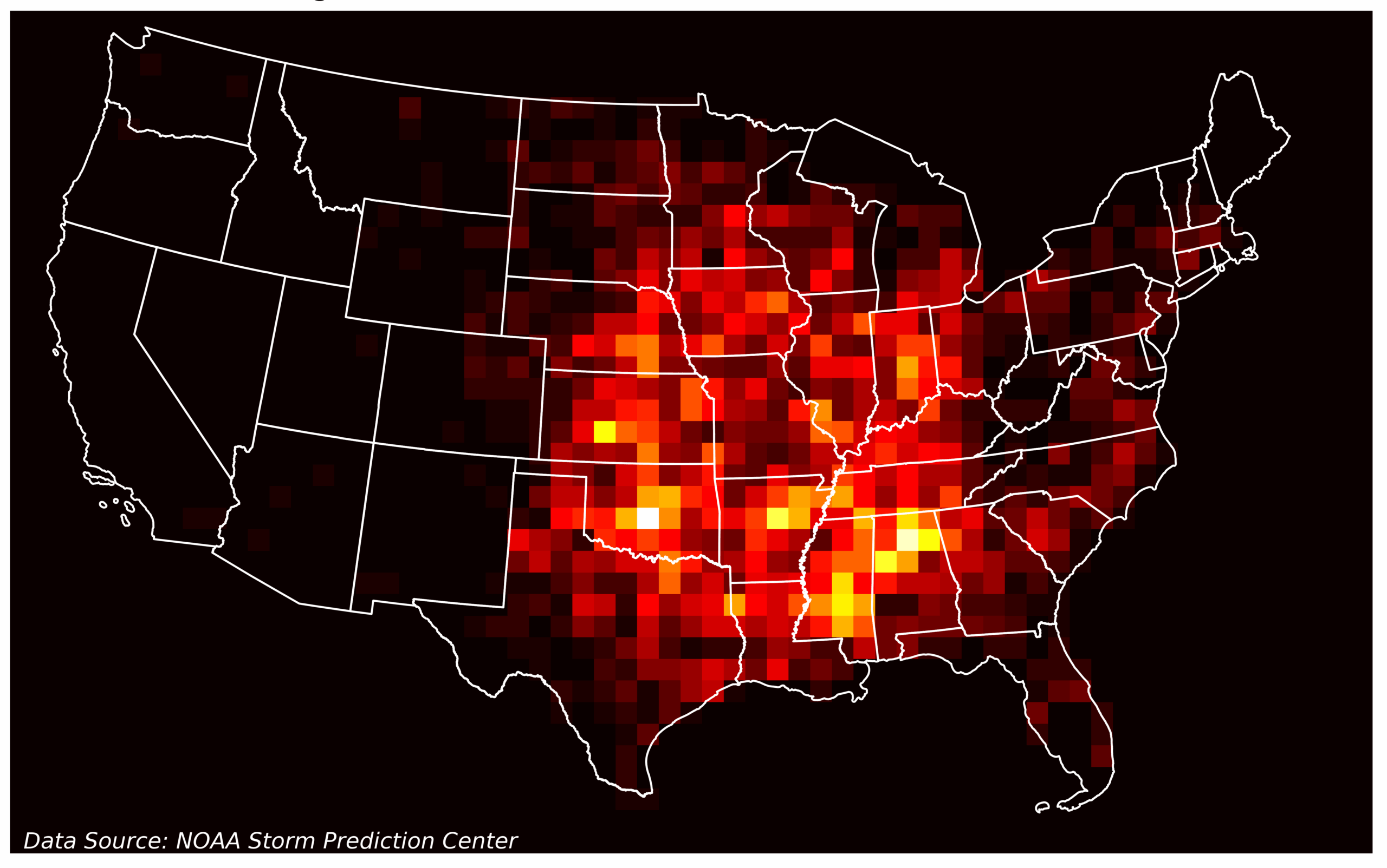
Right here’s the consequence:

The Expanded Code
The next Python code was written in JupyterLab and is described by cell.
Importing Libraries / Assigning Constants
After importing the required libraries, we outline a sequence of configuration constants that enable us to simply alter the filter standards, map boundaries, plot dimensions, and extra. For this evaluation, we concentrate on tornadoes throughout the contiguous United States, filtering out states and territories exterior this space and choosing solely important occasions (these rated EF3 to EF5 on the Enhanced Fujita Scale) from the whole dataset spanning 1950 to 2023. The outcomes are aggregated to 50×50-mile grid cells.
import matplotlib.pyplot as plt
import pandas as pd
import geopandas as gpd
import numpy as np
from shapely.geometry import field


# --- Configuration Constants ---
# Knowledge URLs:
TORNADO_DATA_URL = 'https://bit.ly/40xJCMK'
STATES_DATA_URL = ("https://www2.census.gov/geo/tiger/TIGER2020/STATE/"
                   "tl_2020_us_state.zip")

# Geographic Filtering:
EXCLUDED_STATES_ABBR = ['AK', 'HI', 'PR', 'VI']
TORNADO_MAGNITUDE_FILTER = [3, 4, 5]

# 12 months Filtering (inclusive):
START_YEAR = 1950
END_YEAR = 2023

# Coordinate Reference Methods (CRS):
CRS_LAT_LON = "EPSG:4326"  # WGS 84 geographic CRS (lat/lon)
CRS_ALBERS_EQUAL_AREA = "EPSG:5070"  # NAD83/Conus Albers (projected CRS in m)

# Field for Contiguous US (CONUS) in Albers Equal Space (EPSG:5070 meters):
CONUS_BOUNDS_MIN_X = -2500000
CONUS_BOUNDS_MIN_Y = 100000
CONUS_BOUNDS_MAX_X = 2500000
CONUS_BOUNDS_MAX_Y = 3200000

# Grid Parameters for Heatmap (50x50 mile cells):
GRID_SIZE_MILES = 50
HEATMAP_GRID_SIZE = 80500  # ~50 miles in meters.

# Plotting Configuration:
FIGURE_SIZE = (15, 12)
SAVE_DPI = 600
SAVE_FILENAME = 'tornado_heatmap.png'

# Annotation positions (in EPSG:5070 meters, relative to plot extent):
TITLE_X = CONUS_BOUNDS_MIN_X
TITLE_Y = CONUS_BOUNDS_MAX_Y + 250000  # Offset above max Y
SUBTITLE_X = CONUS_BOUNDS_MIN_X
SUBTITLE_Y = CONUS_BOUNDS_MAX_Y + 100000  # Offset above max Y
SOURCE_X = CONUS_BOUNDS_MIN_X + 50000  # Barely indented from min X
SOURCE_Y = CONUS_BOUNDS_MIN_Y + 20000  # Barely above min Y
Defining Helper Capabilities
The following cell defines two helper capabilities for loading and filtering the dataset and for loading and filtering the state boundaries. Notice that we name on earlier configuration constants in the course of the course of.
# --- Helper Capabilities ---
def load_and_filter_tornado_data():
    """Load information, apply filters, and create a GeoDataFrame."""
    print("Loading and filtering twister information...")
    df_raw = pd.read_csv(TORNADO_DATA_URL)

    # Mix filtering steps into one chained operation:
    masks = (~df_raw['st'].isin(EXCLUDED_STATES_ABBR) &
            df_raw['mag'].isin(TORNADO_MAGNITUDE_FILTER) &
            (df_raw['yr'] >= START_YEAR) & (df_raw['yr'] <= END_YEAR))
    df = df_raw[mask].copy()

    # Create and venture a GeoDataFrame:
    geometry = gpd.points_from_xy(df['slon'], df['slat'],
                                  crs=CRS_LAT_LON)
    temp_gdf = gpd.GeoDataFrame(df, geometry=geometry).to_crs(
                                CRS_ALBERS_EQUAL_AREA)
    return temp_gdf


def load_and_filter_states():
    """Load US state boundaries and filter for CONUS."""
    print("Loading state boundary information...")
    states_temp_gdf = gpd.read_file(STATES_DATA_URL)
    states_temp_gdf = (states_temp_gdf[~states_temp_gdf['STUSPS']
                  .isin(EXCLUDED_STATES_ABBR)].copy())
    states_temp_gdf = states_temp_gdf.to_crs(CRS_ALBERS_EQUAL_AREA)
    return states_temp_gdf
Notice that the tilde (~) in entrance of the masks and states_temp_gdf expressions inverts the outcomes, so we choose rows the place the state abbreviation is not within the excluded record.
Working Helper Capabilities and Producing the Heatmap
The next cell calls the helper capabilities to load and filter the dataset after which clip the information to the map boundaries, generate the heatmap (with the NumPy histogram2d() technique), and outline a steady colormap for the heatmap. Notice that we once more name on earlier configuration constants in the course of the course of.
# --- Knowledge Loading and Preprocessing ---
gdf = load_and_filter_tornado_data()
states_gdf = load_and_filter_states()

# Create bounding field and clip state boundaries & twister factors:
conus_bounds_box = field(CONUS_BOUNDS_MIN_X, CONUS_BOUNDS_MIN_Y,
                       CONUS_BOUNDS_MAX_X, CONUS_BOUNDS_MAX_Y)
clipped_states = gpd.clip(states_gdf, conus_bounds_box)
gdf = gdf[gdf.geometry.within(conus_bounds_box)].copy()

# --- Heatmap Era ---
print("Producing heatmap bins...")
x_bins = np.arange(CONUS_BOUNDS_MIN_X, CONUS_BOUNDS_MAX_X +
                   HEATMAP_GRID_SIZE, HEATMAP_GRID_SIZE)
y_bins = np.arange(CONUS_BOUNDS_MIN_Y, CONUS_BOUNDS_MAX_Y +
                   HEATMAP_GRID_SIZE, HEATMAP_GRID_SIZE)

print("Computing 2D histogram...")
heatmap, x_edges, y_edges = np.histogram2d(gdf.geometry.x,
                                           gdf.geometry.y,
                                           bins=[x_bins, y_bins])

# Outline steady colormap (e.g., 'sizzling', 'viridis', 'plasma', and so forth.):
print("Defining steady colormap...")
cmap = plt.cm.sizzling
norm = None

print("Completed execution.")
As a result of this course of can take a couple of seconds, the print() operate retains us up-to-date on this system’s progress:
Loading and filtering twister information...
Loading state boundary information...
Producing heatmap bins...
Computing 2D histogram...
Defining steady colormap...
Completed execution.
Plotting the Outcomes
The ultimate cell generates and saves the plot. Matplotlib’s imshow() technique is answerable for plotting the heatmap. For extra on imshow(), see this article.
# --- Plotting ---
print("Plotting outcomes...")
fig, ax = plt.subplots(figsize=FIGURE_SIZE)
fig.subplots_adjust(high=0.85)  # Make room for titles.

# Plot state boundaries and heatmap:
clipped_states.plot(ax=ax, shade='none',
                    edgecolor='white', linewidth=1)
vmax = np.max(heatmap)
img = ax.imshow(heatmap.T,
                extent=[x_edges[0], x_edges[-1],
                        y_edges[0], y_edges[-1]],
                origin='decrease',
                cmap=cmap, norm=norm,
                alpha=1.0, vmin=0, vmax=vmax)

# Annotations:
plt.textual content(TITLE_X, TITLE_Y, 'Twister Density Heatmap',
         fontsize=22, fontweight='daring', ha='left')
plt.textual content(x=SUBTITLE_X, y=SUBTITLE_Y, s=(
         f'{START_YEAR}–{END_YEAR}    EF Magnitude 3–5    '
         f'{GRID_SIZE_MILES}×{GRID_SIZE_MILES} mile cells'),
         fontsize=15, ha='left')
plt.textual content(x=SOURCE_X, y=SOURCE_Y,
         s='Knowledge Supply: NOAA Storm Prediction Middle',
         shade='white', fontsize=11,
         fontstyle='italic', ha='left')

# Clear up the axes:
ax.set_xlabel('')
ax.set_ylabel('')
ax.axis('off')

# Put up the Colorbar:
ticks = np.linspace(0, vmax, 6, dtype=int)
cbar = plt.colorbar(img, ax=ax, shrink=0.6, ticks=ticks)
cbar.set_label('nTornado Depend per Grid Cell', fontsize=15)
cbar.ax.set_yticklabels(record(map(str, ticks)))

print(f"Saving plot as '{SAVE_FILENAME}'...")
plt.savefig(SAVE_FILENAME, bbox_inches='tight', dpi=SAVE_DPI)
print("Plot saved.n")
plt.present()
This produces the next map:

It is a lovely map and extra informative than a {smooth} KDE different.
Including Twister Ending Places
Our twister density heatmaps are primarily based on the beginning places of tornadoes. However tornadoes transfer after touching down. The typical twister monitor is about 3 miles lengthy, however whenever you have a look at stronger storms, the numbers enhance. EF‑3 tornadoes common 18 miles, and EF‑4 tornadoes common 27 miles. Lengthy-track tornadoes are uncommon, nevertheless, comprising less than 2% of all tornadoes.
As a result of the typical twister monitor size is lower than the 50-mile dimension of our grid cells, we are able to anticipate them to cowl just one or two cells on the whole. Thus, together with the twister ending location ought to assist us enhance our density measurement.
To do that, we’ll want to mix the beginning and ending lat-lon places and filter out endpoints that share the similar cell as their corresponding beginning factors. In any other case, we’ll “double-dip” when counting. The code for it is a bit lengthy, so I’ve saved it on this Gist.
Right here’s a comparability of the “begin solely” map with the mixed beginning and ending places:

The prevailing winds drive most tornadoes towards the east and northeast. You may see the influence in states like Missouri, Mississippi, Alabama, and Tennessee. These areas have brighter cells within the backside map because of tornadoes beginning in a single cell and ending within the adjoining easterly cell. Notice additionally that the utmost variety of tornadoes in a given cell has elevated from 29 (within the higher map) to 33 (within the backside map).
Recap
We used Python, pandas, GeoPandas, and Matplotlib to venture and overlay heatmaps onto geographical maps. Geospatial heatmaps are a extremely efficient solution to visualize regional tendencies, patterns, hotspots, and outliers in statistical information.
For those who get pleasure from some of these initiatives, be sure you take a look at my e-book, Real World Python: A Hacker’s Guide to Solving Problems with Code, out there in bookstores and on-line.

